One of the exciting benefits of analyzing literary data is that it can be visualized! I have included some of my favorite visualizations made with the data taken from the works that we used in our analysis. The visualizations were created in RStudio, with the R programming language.
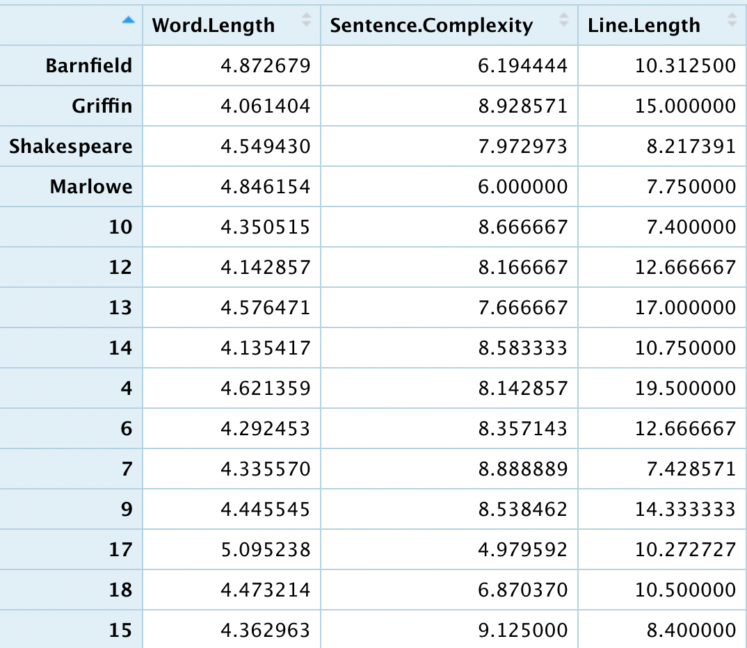
For reference, here is the data table I worked with:
Here, I plotted the unknown poems from The Passionate Pilgrim (listed by the number they appear under in the text) as well as the confirmed works of the 4 potential authors.

I noticed that there seemed to be a downward correlation between word length and sentence complexity in the works. The red line in the graph below is a linear regression line that shows that correlation.

The implication of this finding is that when the poets used longer words, they used less punctuation in their sentences. It is as if punctuation or word length made their writing more complex, so if one was high, the other didn’t have to be.
The following bivariate boxplot illustrates how one poem, XVII (or 17), is a significant outlier in the comparison between sentence complexity and word length, with a very high average word length and a very low sentence complexity.
Note: Bivariate boxplots represent 2-dimensional data, with the inner dotted circle (called the hinge) denoting where the first 50% of the data ends, and the outer circle (called the fence) denotes where the non-outlier data ends.
To check out whether the outlier-ship of poem XVII makes sense, the first 8 lines are printed below:
My flocks feed not,
My ewes breed not,
My rams speed not,
All is amiss:
Love is dying,
Faith’s defying,
Heart’s denying,
Causer of this.
The lines in poem XVII are very short, but the author’s vocabulary is not noticeably different than the other poems. Hence, the low sentence complexity.
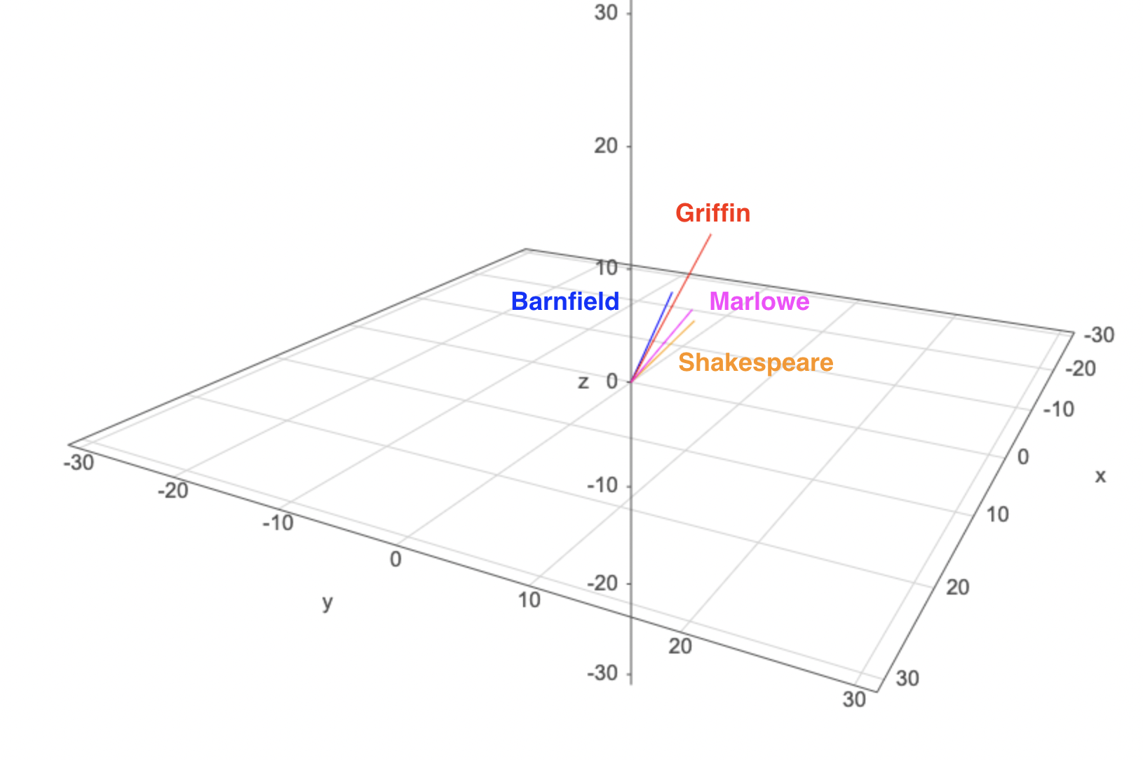
Since the authorship analysis was based mostly on 3 variables (line length, word length, and sentence complexity) it is worth representing all 3 of them in a plot. That is what the 3d scatterplot below does. All of the unknown works are represented.

Using the three attributes, poem/author fingerprints can be plotted as vectors as well as points. Note how each vector points in a similar direction, indicating that the relationship between the three attributes is quite similar for all 4 authors. This makes sense, since they were all contemporaries.
If you look closely, you can also see that Griffin and Barnfield appear to cluster together and Marlowe and Shakespeare do the same. I note in the project reflection that almost all (4/5) of the differences between our classifications and those of Elliott and Valenza (1991) are that we attribute a poem to Marlowe when they found it within Shakespeare’s statistical range.
Now for some fun stuff: humans are quite good at identifying visual similarities between shapes.
The following star plots display the three attributes in the data table by extending a line out to the magnitude of the attribute for the specific row. The size of the plot indicates the magnitude of all 3 attributes (e.g., Poem 4 has a relatively high word length, line length, and sentence complexity), while the shape indicates the relationship between the attributes.

Plots that look similar have similar attributes. For example, Poems 12 and 14 look quite similar in these plots, and our model classified both as being written by Bartholomew Griffin.
The final visualization is a series of Chernoff faces, a technique that maps each column of the data table to a characteristic of the face (e.g., the shade of the face color corresponds to the average word length). This allows the viewer to perceive patterns that would otherwise be difficult to see
For example, the “Griffin” face is very similar to the face for Poem 12, and indeed, through our analysis we found with confidence that Poem 12 was written by Bartholomew Griffin.